
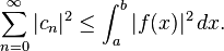
http://en.wikipedia.org/wiki/List_of_computer_system_emulators
Hello to every one in this section i willl cover an interesting topic useful for people who write machine code emulators if this is your case this article can be useful to you in order to optimize speed at runtime ie to emulate a x8086 in an iphone that goes at pretty 1Ghz.
lets see some debug code of the game Raven at asm:
; 45   :   if (isReadyForNextShot())

        mov     ecx, DWORD PTR _this$[ebp]
        call    ?isReadyForNextShot@Raven_Weapon@@IAE_NXZ ; Raven_Weapon::isReadyForNextShot
        movzx   eax, al
        test    eax, eax
        je      SHORT $LN1@ShootAt

; 46   :   {
; 47   :     //fire!
; 48   :     m_pOwner->GetWorld()->AddBolt(m_pOwner, pos);

        sub     esp, 16                                 ; 00000010H
        mov     ecx, esp
        mov     edx, DWORD PTR _pos$[ebp]
        mov     DWORD PTR [ecx], edx
        mov     eax, DWORD PTR _pos$[ebp+4]
        mov     DWORD PTR [ecx+4], eax
        mov     edx, DWORD PTR _pos$[ebp+8]
        mov     DWORD PTR [ecx+8], edx
        mov     eax, DWORD PTR _pos$[ebp+12]
        mov     DWORD PTR [ecx+12], eax
        mov     ecx, DWORD PTR _this$[ebp]
        mov     edx, DWORD PTR [ecx+8]
        push    edx
        mov     eax, DWORD PTR _this$[ebp]
        mov     ecx, DWORD PTR [eax+8]
        call    ?GetWorld@Raven_Bot@@QAEQAVRaven_Game@@XZ ; Raven_Bot::GetWorld
        mov     ecx, eax
        call    ?AddBolt@Raven_Game@@QAEXPAVRaven_Bot@@UVector2D@@@Z ; Raven_Game::AddBolt
and now we can substitute our asm code for another layer that goes between machine-code and asm not already compiled so the calls are being substitute by machine codeand the variables also.
the layer of the implemented language that should be developed by you will remember you sql if at sometime you have work with databases.the idea is to have one stack per type of machine code instruction independently of the registers,mem,
indirection mem of the instruction
the result of the saw asm code is:
select esp-16,ecx=(select esp,esp_1 from mov1,sub1 where sub1.esp-16=mov1.esp),
edx=(select PTR_pos$[ebp+4] from mov2 where PTR_pos$[ebp+4]=mov2.PTR_pos$[ebp+4]
*/in this case can be ommited*/ ),
DWORD PTR[ecx+4]=(select eax from mov3 where ...) from mov_general
etc
this is not a nice example but if caller procedure
?GetWorld@Raven_Bot@@QAEQAVRaven_Game@@XZ ; Raven_Bot::GetWorld
what to do it is to add 10 to eax and then make a jne to jump to anywhere
we can being complicating the query so:
select esp-16,ecx=(select esp,esp_1 from mov1,sub1 where sub1.esp-16=mov1.esp),
edx=(select PTR_pos$[ebp+4] from mov2 where PTR_pos$[ebp+4]=mov2.PTR_pos$[ebp+4]
*/in this case can be ommited*/ ),
DWORD PTR[ecx+4]=(select eax from mov3 where mov3.eax=add.eax),DWORD PTR[ecx+4]+10as eax_plus_10 from mov_general where DWORD PTR[ecx+4]+10<0  <0 is jne asm instruction condition matched
if you take a deep inspection at the select you will quickly realize that evaluating from left registers to rightmost from top to down you obtain a step sequence ofthe asm code that can be debugged throught the interpretation of the select clausetake in one step per step.
probably at the beginning could look like a very nasty task to create code to go
making growing the select clause more and more until some kind of instruction likean out or int can't be parsed but with the help of some c,c++,c# switch instruction an stack of pointers per instruction per "stack" mov[i]->eax ,sub[i]->eax making some comparisons for where typeof(mov[0]->eax)==typeof(sub[2]->eax)&&
mov[0]->eax==sub[2]->eax etc.

and with and LL(n) parser to rearrange clauses i let you to your imagination can be cool to implement it.
When the parser starts, the stack already contains two symbols:
[ S, $ ]
where '$' is a special terminal to indicate the bottom of the stack and the end of the input stream, and 'S' is the start symbol of the grammar. The parser will attempt to rewrite the contents of this stack to what it sees on the input stream. However, it only keeps on the stack what still needs to be rewritten.
[edit]Concrete example
[edit]Set up
To explain its workings we will consider the following small grammar:
- S → F selectallclause1 eax=10->F eax=10
- S → ( S + F ) selectclause1 eax=10->(selectclause1 eax=10)+F eax=20
- F → a Feax=a
and parse the following input:
- ( a + a ) a+a=10+10
The parsing table for this grammar looks as follows:
( ) a + $ S 2 - 1 - - F - - 3 - -
(S+F)*2due dont exist op * we simplify (S+F)+(S+F)=F+F=4 1+3=a+a
(Note that there is also a column for the special terminal, represented here as $, that is used to indicate the end of the input stream.)
[edit]Parsing procedure
In each step, the parser reads the next-available symbol from the input stream, and the top-most symbol from the stack. If the input symbol and the stack-top symbol match, the parser discards them both, leaving only the unmatched symbols in the input stream and on the stack.
Thus, in its first step, the parser reads the input symbol '(' and the stack-top symbol 'S'. The parsing table instruction comes from the column headed by the input symbol '(' and the row headed by the stack-top symbol 'S'; this cell contains '2', which instructs the parser to apply rule (2). The parser has to rewrite 'S' to '( S + F )' on the stack and write the rule number 2 to the output. The stack then becomes:
[ (, S, +, F, ), $ ]
Since the '(' from the input stream did not match the top-most symbol, 'S', from the stack, it was not removed, and remains the next-available input symbol for the following step.
In the second step, the parser removes the '(' from its input stream and from its stack, since they match. The stack now becomes:
[ S, +, F, ), $ ]
Now the parser has an 'a' on its input stream and an 'S' as its stack top. The parsing table instructs it to apply rule (1) from the grammar and write the rule number 1 to the output stream. The stack becomes:
[ F, +, F, ), $ ]
The parser now has an 'a' on its input stream and an 'F' as its stack top. The parsing table instructs it to apply rule (3) from the grammar and write the rule number 3 to the output stream. The stack becomes:
[ a, +, F, ), $ ]
In the next two steps the parser reads the 'a' and '+' from the input stream and, since they match the next two items on the stack, also removes them from the stack. This results in:
[ F, ), $ ]
In the next three steps the parser will replace 'F' on the stack by 'a', write the rule number 3 to the output stream and remove the 'a' and ')' from both the stack and the input stream. The parser thus ends with '$' on both its stack and its input stream.
In this case the parser will report that it has accepted the input string and write the following list of rule numbers to the output stream:
- [ 2, 1, 3, 3 ]
This is indeed a list of rules for a leftmost derivation of the input string, which is:
- S → ( S + F ) → ( F + F ) → ( a + F ) → ( a + a )
note you can construct the parse with some thing like this
http://en.wikipedia.org/wiki/LL_parser
#include
This is indeed a list of rules for a leftmost derivation of the input string, which is:
- S → ( S + F ) → ( F + F ) → ( a + F ) → ( a + a )
-
-
Emulator
From Wikipedia, the free encyclopedia
This article is about emulators in computer science. For a line of digital musical instruments, see E-mu Emulator. For other uses, see Emulation (disambiguation).
An emulator in computer sciences duplicates (provides an emulation of) the functions of one system using a different system, so that the second system behaves like (and appears to be) the first system. This focus on exact reproduction of external behavior is in contrast to some other forms of computer simulation, which can concern an abstract model of the system being simulated.
[edit]Emulators in computer science
Emulation refers to the ability of a computer program or electronic device to imitate another program or device. Many printers, for example, are designed to emulate Hewlett-Packard LaserJet printers because so much software is written for HP printers. If a non-HP printer emulates an HP printer, any software written for a real HP printer will also run in the non-HP printer emulation and produce equivalent printing.
A hardware emulator is an emulator which takes the form of a hardware device. Examples include the DOS-compatible card installed in some old-world Macintoshes like Centris 610 or Performa 630 that allowed them to run PC programs and FPGA-based hardware emulators.
In a theoretical sense, the Church-Turing thesis implies that any operating environment can be emulated within any other. However, in practice, it can be quite difficult, particularly when the exact behavior of the system to be emulated is not documented and has to be deduced through reverse engineering. It also says nothing about timing constraints; if the emulator does not perform as quickly as the original hardware, the emulated software may run much more slowly than it would have on the original hardware, possibly triggering time interrupts to alter performance.
[edit]Emulation in preservation
Emulation is a strategy in digital preservation to combat obsolescence. Emulation focuses on recreating an original computer environment, which can be time-consuming and difficult to achieve, but valuable because of its ability to maintain a closer connection to the authenticity of the digital object.[1]
Emulation addresses the original hardware and software environment of the digital object, and recreates it on a current machine.[2] The emulator allows the user to have access to any kind of application oroperating system on a current platform, while the software runs as it did in its original environment.[3] Jeffery Rothenberg, an early proponent of emulation as a digital preservation strategy states, “the ideal approach would provide a single extensible, long-term solution that can be designed once and for all and applied uniformly, automatically, and in synchrony (for example, at every refresh cycle) to all types of documents and media”.[4] He further states that this should not only apply to out of date systems, but also be upwardly mobile to future unknown systems.[5] Practically speaking, when a certain application is released in a new version, rather than address compatibility issues and migration for every digital object created in the previous version of thatapplication, one could create an emulator for the application, allowing access to all of said digital objects.
[edit]Benefits
- Emulators maintain the original look, feel, and behavior of the digital object, which is just as important as the digital data itself.[6]
- Despite the original cost of developing an emulator, it may prove to be the more cost efficient solution over time.[7]
- Reduces labor hours, because rather than continuing an ongoing task of continual data migration for every digital object, once the library of past and present operating systems and application software is established in an emulator, these same technologies are used for every document using those platforms.[3]
- Many emulators have already been developed and released under GNU General Public License through the open source environment, allowing for wide scale collaboration.[8]
- Emulators allow video games exclusive to one system to be played on another. For example, Uncharted 2, a PS3 exclusive game, could (in theory) be played on a PC or Xbox 360 using an emulator.
[edit]Obstacles
- Intellectual property - Many technology vendors implemented non-standard features during program development in order to establish their niche in the market, while simultaneously applying ongoing upgrades to remain competitive. While this may have advanced the technology industry and increased vendor’s market share, it has left users lost in a preservation nightmare with little supporting documentation due to the proprietary nature of the hardware and software.[9]
- Copyright laws are not yet in effect to address saving the documentation and specifications of proprietary software and hardware in an emulator module.[10]
[edit]Emulators in new media art
Because of its primary use of digital formats, new media art relies heavily on emulation as a preservation strategy. Artists such as Cory Arcangel specialize in resurrecting obsolete technologies in their artwork and recognize the importance of a decentralized and deinstitutionalized process for the preservation of digital culture.
In many cases, the goal of emulation in new media art is to preserve a digital medium so that it can be saved indefinitely and reproduced without error, so that there is no reliance on hardware that ages and becomes obsolete. The paradox is that the emulation and the emulator have to be made to work on future computers.[11]
[edit]Types of emulators
Most emulators just emulate a hardware architecture—if operating system firmware or software is required for the desired software, it must be provided as well (and may itself be emulated). Both the OS and the software will then be interpreted by the emulator, rather than being run by native hardware. Apart from this interpreter for the emulated binary machine's language, some other hardware (such as input or output devices) must be provided in virtual form as well; for example, if writing to a specific memory location should influence what is displayed on the screen, then this would need to be emulated.
While emulation could, if taken to the extreme, go down to the atomic level, basing its output on a simulation of the actual circuitry from a virtual power source, this would be a highly unusual solution. Emulators typically stop at a simulation of the documented hardware specifications and digital logic. Sufficient emulation of some hardware platforms requires extreme accuracy, down to the level of individual clock cycles, undocumented features, unpredictable analog elements, and implementation bugs. This is particularly the case with classic home computers such as the Commodore 64, whose software often depends on highly sophisticated low-level programming tricks invented by game programmers and the demoscene.
In contrast, some other platforms have had very little use of direct hardware addressing. In these cases, a simple compatibility layer may suffice. This translates system calls for the emulated system into system calls for the host system e.g., the Linux compatibility layer used on *BSD to run closed source Linux native software on FreeBSD, NetBSD and OpenBSD.
Developers of software for embedded systems or video game consoles often design their software on especially accurate emulators called simulators before trying it on the real hardware. This is so that software can be produced and tested before the final hardware exists in large quantities, so that it can be tested without taking the time to copy the program to be debugged at a low level and without introducing the side effects of a debugger. In many cases, the simulator is actually produced by the company providing the hardware, which theoretically increases its accuracy.
Math coprocessor emulators allow programs compiled with math instructions to run on machines that don't have the coprocessor installed, but the extra work done by the CPU may slow the system down. If a math coprocessor isn't installed or present on the CPU, when the CPU executes any coprocessor instruction it will make a determined interrupt (coprocessor not available), calling the math emulator routines. When the instruction is successfully emulated, the program continues executing.
[edit]Structure of an emulator

This article's section named "Structure of an emulator" does not cite any references or sources. Please help improve this article by adding citations to reliable sources. Unsourced material may be challenged and removed. (June 2008)
Typically, an emulator is divided into modules that correspond roughly to the emulated computer's subsystems. Most often, an emulator will be composed of the following modules:
- a CPU emulator or CPU simulator (the two terms are mostly interchangeable in this case)
- a memory subsystem module
- various I/O devices emulators
Buses are often not emulated, either for reasons of performance or simplicity, and virtual peripherals communicate directly with the CPU or the memory subsystem.
[edit]Memory subsystem
It is possible for the memory subsystem emulation to be reduced to simply an array of elements each sized like an emulated word; however, this model falls very quickly as soon as any location in the computer's logical memory does not match physical memory.
This clearly is the case whenever the emulated hardware allows for advanced memory management (in which case, the MMU logic can be embedded in the memory emulator, made a module of its own, or sometimes integrated into the CPU simulator).
Even if the emulated computer does not feature an MMU, though, there are usually other factors that break the equivalence between logical and physical memory: many (if not most) architecture offer memory-mapped I/O; even those that do not almost invariably have a block of logical memory mapped to ROM, which means that the memory-array module must be discarded if the read-only nature of ROM is to be emulated. Features such as bank switching or segmentation may also complicate memory emulation.
As a result, most emulators implement at least two procedures for writing to and reading from logical memory, and it is these procedures' duty to map every access to the correct location of the correct object.
On a base-limit addressing system where memory from address 0 to address ROMSIZE-1 is read-only memory, while the rest is RAM, something along the line of the following procedures would be typical:
void WriteMemory(word Address, word Value) {
word RealAddress;
RealAddress = Address + BaseRegister;
if ((RealAddress < LimitRegister) &&
(RealAddress > ROMSIZE)) {
Memory[RealAddress] = Value;
} else {
RaiseInterrupt(INT_SEGFAULT);
}
}
word ReadMemory(word Address) {
word RealAddress;
RealAddress=Address+BaseRegister;
if (RealAddress < LimitRegister) {
return Memory[RealAddress];
} else {
RaiseInterrupt(INT_SEGFAULT);
return NULL;
}
}
[edit]CPU simulator
The CPU simulator is often the most complicated part of an emulator. Many emulators are written using "pre-packaged" CPU simulators, in order to concentrate on good and efficient emulation of a specific machine.
The simplest form of a CPU simulator is an interpreter, which follows the execution flow of the emulated program code and, for every machine code instruction encountered, executes operations on the host processor that are semantically equivalent to the original instructions.
This is made possible by assigning a variable to each register and flag of the simulated CPU. The logic of the simulated CPU can then more or less be directly translated into software algorithms, creating a software re-implementation that basically mirrors the original hardware implementation.
The following example illustrates how CPU simulation can be accomplished by an interpreter. In this case, interrupts are checked-for before every instruction executed, though this behavior is rare in real emulators for performance reasons.
void Execute(void) {
if (Interrupt != INT_NONE) {
SuperUser = TRUE;
WriteMemory(++StackPointer, ProgramCounter);
ProgramCounter = InterruptPointer;
}
switch (ReadMemory(ProgramCounter++)) {
/*
* Handling of every valid instruction
* goes here...
*/
default:
Interrupt = INT_ILLEGAL;
}
}
Interpreters are very popular as computer simulators, as they are much simpler to implement than more time-efficient alternative solutions, and their speed is more than adequate for emulating computers of more than roughly a decade ago on modern machines.
However, the speed penalty inherent in interpretation can be a problem when emulating computers whose processor speed is on the same order of magnitude as the host machine. Until not many years ago, emulation in such situations was considered completely impractical by many.
What allowed breaking through this restriction were the advances in dynamic recompilation techniques. Simple a priori translation of emulated program code into code runnable on the host architecture is usually impossible because of several reasons:
- code may be modified while in RAM, even if it is modified only by the emulated operating system when loading the code (for example from disk)
- there may not be a way to reliably distinguish data (which should not be translated) from executable code.
Various forms of dynamic recompilation, including the popular Just In Time compiler (JIT) technique, try to circumvent these problems by waiting until the processor control flow jumps into a location containing untranslated code, and only then ("just in time") translates a block of the code into host code that can be executed. The translated code is kept in a code cache, and the original code is not lost or affected; this way, even data segments can be (meaninglessly) translated by the recompiler, resulting in no more than a waste of translation time.
Speed may not be desirable as some older games were not designed with the speed of faster computers in mind. A game designed for a 30 MHz PC with a level timer of 300 game seconds might only give the player 30 seconds on a 300 MHz PC. Other programs, such as some DOS programs, may not even run on faster computers. Particularly when emulating computers which were "closed-box", in which changes to the core of the system were not typical, software may use techniques that depend on specific characteristics of the computer it ran on (i.e. its CPU's speed) and thus precise control of the speed of emulation is important for such applications to be properly emulated.
[edit]I/O
Most emulators do not, as mentioned earlier, emulate the main system bus; each I/O device is thus often treated as a special case, and no consistent interface for virtual peripherals is provided.
This can result in a performance advantage, since each I/O module can be tailored to the characteristics of the emulated device; designs based on a standard, unified I/O API can, however, rival such simpler models, if well thought-out, and they have the additional advantage of "automatically" providing a plug-in service through which third-party virtual devices can be used within the emulator.
A unified I/O API may not necessarily mirror the structure of the real hardware bus: bus design is limited by several electric constraints and a need for hardware concurrency management that can mostly be ignored in a software implementation.
Even in emulators that treat each device as a special case, there is usually a common basic infrastructure for:
- managing interrupts, by means of a procedure that sets flags readable by the CPU simulator whenever an interrupt is raised, allowing the virtual CPU to "poll for (virtual) interrupts"
- writing to and reading from physical memory, by means of two procedures similar to the ones dealing with logical memory (although, contrary to the latter, the former can often be left out, and direct references to the memory array be employed instead)
[edit]Emulation versus simulation
The word "emulator" was coined in 1957 at IBM, as an optional feature in the IBM 709 to execute legacy IBM 704 programs on the IBM 709. Registers and most 704 instructions were emulated in 709 hardware. Complex 704 instructions such as floating point trap and input-output routines were emulated in 709 software. In 1963, IBM constructed emulators for development of the NPL (360) product line, for the "new combination of software, microcode, and hardware".[12]
It has recently become common to use the word "emulate" in the context of software. However, before 1980, "emulation" referred only to emulation with a hardware or microcode assist, while "simulation" referred to pure software emulation.[13] For example, a computer specially built for running programs designed for another architecture is an emulator. In contrast, a simulator could be a program which runs on a PC, so that old Atari games can be run on it. Purists continue to insist on this distinction, but currently the term "emulation" often means the complete imitation of a machine executing binary code.
[edit]Logic simulators
Main article: Logic simulation
Logic simulation is the use of a computer program to simulate the operation of a digital circuit such as a processor. This is done after a digital circuit has been designed in logic equations, but before the circuit is fabricated in hardware.
[edit]Functional simulators
Main article: High level emulation
Functional simulation is the use of a computer program to simulate the execution of a second computer program written in symbolic assembly language or compiler language, rather than in binary machine code. By using a functional simulator, programmers can execute and trace selected sections of source code to search for programming errors (bugs), without generating binary code. This is distinct from simulating execution of binary code, which is software emulation.
The first functional simulator was written by Autonetics about 1960 for testing assembly language programs for later execution in military computer D-17B. This was so that flight programs could be written, executed, and tested before D-17B computer hardware had been built. Autonetics also programmed a functional simulator for testing flight programs for later execution in the military computer D-37C.
[edit]Video game console emulators
Main article: Video game console emulator
Video game console emulators are programs that allow a computer or modern console to emulate a video game console. They are most often used to play older video games on personal computers and modern video game consoles, but they are also used to translate games into other languages, to modify existing games, and in the development process of home brew demos and new games for older systems. The internet has helped in the spread of console emulators, as most - if not all - would be unavailable for sale in retail outlets. Examples of console emulators that have been released in the last 2 decades are: Zsnes, Kega Fusion, Desmume, Epsxe, Project64, Visual Boy Advance, NullDC and Nestopia.
[edit]Terminal emulators
Main article: Terminal emulator
Terminal emulators are software programs that provide modern computers and devices interactive access to applications running on mainframe computer operating systems or other host systems such as HP-UX or OpenVMS. Terminals such as the IBM 3270 or VT100 and many others, are no longer produced as physical devices. Instead, software running on modern operating systems simulates a "dumb" terminal and is able to render the graphical and text elements of the host application, send keystrokes and process commands using the appropriate terminal protocol. Some terminal emulation applications include Attachmate Reflection, IBM Personal Communications, Stromasys CHARON-VAX/AXP and Micro Focus Rumba.
[edit]Legal controversy
- See article Console emulator — Legal issues
[edit]See also
- The list of emulators
- The list of computer system emulators
- Computer simulation is the larger field of modeling real-world phenomenon (e.g. physics and economy) using computers.
- For rewriting a computer program into a different programming language or platform, see Porting.
- Field-programmable gate arrays (FPGAs)
- Other uses of the term "emulator" in the field of computer science:
- Logic simulation
- Functional simulation
- Translation:
- QEMU
- Q (emulator)
- Hardware emulation
- Hardware-assisted virtualization
- Virtual machine
- MAME
- data migration
- backward compatibility
- forward compatibility
[edit]References
- ^ "What is emulation?". Koninklijke Bibliotheek. Retrieved 2007-12-11.
- ^ van der Hoeven, Jeffrey, Bram Lohman, and Remco Verdegem. “Emulation for Digital Preservation in Practice: The Results.” The International Journal of Digital Curation 2.2 (2007): 123-132.
- ^ a b Muira, Gregory. “ Pushing the Boundaries of Traditional Heritage Policy: maintaining long-term access to multimedia content.” IFLA Journal 33 (2007): 323-326.
- ^ Rothenberg, Jeffrey (1998). "“Criteria for an Ideal Solution.” Avoiding Technological Quicksand: Finding a Viable Technical Foundation for Digital Preservation.". Council on Library and Information Resources. Washington, DC.
- ^ Rothenberg, Jeffrey. “The Emulation Solution.” Avoiding Technological Quicksand: Finding a Viable Technical Foundation for Digital Preservation. Washington, DC: Council on Library and Information Resources, 1998. Council on Library and Information Resources. 2008. 28 Mar. 2008 http://www.clir.org/pubs/reports/rothenberg/contents.html
- ^ Muira, Gregory. “ Pushing the Boundaries of Traditional Heritage Policy: maintaining long-term access to multimedia content.” IFLA Journal 33 (2007): 323-326.
- ^ Granger, Stewart. Digital Preservation & Emulation: from theory to practice. Proc. of the ichim01 Meeting, vol. 2, 3 -7 Sept. 2001. Milano, Italy. Toronto: Archives and Museum Informatics, University of Toronto, 2001. 28 Mar. 2008http://www.leeds.ac.uk/cedars/pubconf/papers/ichim01SG.html
- ^ van der Hoeven, Jeffrey, Bram Lohman, and Remco Verdegem. “Emulation for Digital Preservation in Practice: The Results.” The International Journal of Digital Curation 2.2 (2007): 123-132.
- ^ Granger, Stewart. “Emulation as a Digital Preservation Strategy.” D-Lib Magazine 6.19 (2000). 29 Mar 2008 http://www.dlib.org/dlib/october00/granger/10granger.html
- ^ Rothenberg, Jeffrey. “The Emulation Solution.” Avoiding Technological Quicksand: Finding a Viable Technical Foundation for Digital Preservation. Washington, DC: Council on Library and Information Resources, 1998. Council on Library and Information Resources. 2008. 28 Mar. 2008
- ^ "Echoes of Art: Emulation as preservation strategy". Retrieved 2007-12-11.
- ^ Pugh, Emerson W.; et al. (1991). IBM's 360 and Early 370 Systems. MIT. ISBN 0-262-16123-0. pages 160-161
- ^ S. G. Tucker, "Emulation of Large Systems", Communications of the ACM (CACM) Vol. 8, No. 12, Dec. 1965, pp. 753-761
[edit]External links
- Emuwiki.com is a repertory of emulators and their respective histories.
- Emulator at the Open Directory Project


ARCHITECTURING OLD .NET REMOTING SERVICES.
Extracted from the book .NET PATTERNS Architecture , Design and Process by Christian Thilmany
Remote Tracing - Building a Remote Trace Listener
When we work with remoting objects just before to put into production our Serviced Aplication we need to detect wich one was the exact failure to notify (to the Admnistrator) to the server part if the execution error was raised at UI part of our at least two tier application or if an exception is raised in the server part due a Database Error it also can be handled in a general exception treatment to notify that that action cant be temporarily performed the problem cant be addressed as a general whole try catch block due the boundaries of our two tier are separated into a client UI interface plus at least a second Bussiness-DataAccess tier its needed to contruct a trace Listener and to fulfill remote tracing code we can enhance this in many forms but one of them is to create a Custom Trace Listener, a Trace Receiver and a Trace Viewer.
we can create Two Trace Listeners with different key one that goes from server tier to UI and another that goes in the inverse direction from UI to BUsiness-DataAccess components to a MSMQ to later save into a database store in eventlog on the server or send a Mail to an Administrator, its as well needed two receivers in the same way from server to UI must be trapped the exeption locally resend to UI the Tracemessage and rethrow the exception in a bubble up pattern so it reaches a general exception manager that sends the message finally to a general method of the UI, the inverse problem appears when form UI we should resend the Exception to the main remote server.
Building a Custom Trace Listener:
we need to edit config.cs
<system.diagnostics>
. <switches>
<add name="RemoteTRaceLevel" value="1" />
<switches>
</system.diagnostics>
0 off ,1 error , 2 warning , 3 info , 4 verbose
in remote components you just have to make accessible to that execution boundary to the following code classes:
public class RemoteTraceListener:System.Diagnostics.TraceListener
{
private RemoteTraceServer oRemoteService=null;
public RemoteTracerService RemoteService
{
get { return oRemoteService; }
set { oRemoteService = value; }
}
public RemoteTraceListener(string sName)
{
RemoteService = new RemoteTraceService();
base.Name=sName;
}
public override void Write(string sMessage)
{
RemoteService.RemoteTrace(Dns.GetHostName(),sMessage);
}
public override WRiteLine(string sMEssage)
{
RemoteSErvice.RemoteTrace(Dns.GetHostName(), sMessage);
}
then in the remote code you just have to call instead of Trace.write or Trace.WriteLine,-> RemoteSErvice.RemoteTrace(Message)
a.1) Sample Routine for constructing and adding your custom Listener
public static void InitTraceListeners()
{
If(Trace.Listeners[TRACE_REMOTE_LISTENER_KEY]==null)
Trace.Listeners.Add(new RemoteTraceListener(TRACE_REMOTE_LISTENER_KEY); this should be done per remote componenr
}
Sample Business Object to be placed on a queue.
public struct BUsinessMessage
{
private string sType;
private string UserId;
...
private string sQueueName;
private string sMessageText;
private string sDate;
private string sTime;
public string MessageType
{
get {return sType;}
set
{
sType=value;
sQueueName=".\\private$\\test" +sType.ToLower();
}
}
public string MessageText
{
get { return sMessageText;}
set {sMessageText=value;}
}
public string Date
{
get{ return sDate;}
set{sDate=value;}
}
...
public string UserId
{
get{return sUserId;}
set{sUserId=value;}
}
public string QueueName
{
get{return sQueueName;}
}
}
public class Messenger
{
private BusinessMEssge oMessage;
public BusinessMessage MessageInfo
{
get {return oMessage;}
set {oMessage=value;}
}
public Messnger()
{
MessageInfo = new BUsinessMessage();
}
public void Send(BusinessMessage oMessage)
{
MessageInfo= oMessage;
Send();
}
public void Send()
{
try
{
string sQueuePath=MessageInfo.QueueName;
if(!MessageQueue.Exists(SQueuePath))
{
MessageQueue.Create(SQueuePath);
}
MessageQueue oQueue = new MessageQueue(sQueuePath);
OQueue,Send(MessageInfo.MessageType + "-" + MessageInfo.Uri);
}
catch (Exception e)
{
throw new BaseException(this,0,e.Messge,e,false);
}
}
public BusinessMessage Receive(BUsinessMessage oMessage, int nTimeOut)
{
MessageInfo= oMessage;
return Receive(nTimeOut);
}
public BusinessMessge Receive(int nTimeOut)
{
try
{
string sQueuePath=MEssageInfo.QueueName;
if(!MessageQueue.Exists(sQueuePAth))
{
//Queue doesnot exists so threw an exception
throw new Exception("Receive-Error"+sQueuePath+" queue doesnot exists.");
}
MessageQueue oQueu = new MessageQueue(SQueuePath);
((xmlMessageFormatter)oQueueFormatter).TargetTypes=new Type[]{typeof(BussinessMessge));
System.Messaging.Message oRawMessage = oQueue.Receive(new TimeSpan(0,0,nTimeoOut));
BusinessMessage o MessageBody=(BusinessMessage)oRAwMessage.Body;
MessageInfo=oMessageBody;
}
catch(Exception e)
{
throw new BaseException(this,0,e.Message,e,false);
}
}
b) Sending Traces via Sockets:
I also send the trace to a socket server on the network.I do this setting my host,ip,port and calling my utility method Utilities.SendSocketStream.This methosd creates a connection with the specified host and if succesful , sebnds the trace message as a byte stream.
b.1)Sample Socket Routine for sending any message.
public static string SendSocketStream(string sHost,int nPort,string Message)
{
TcpClient oTcpClient=null;
string sAck=null;
int nBytesRead=0;
NetworkStream oStream=null;
try
{
oTcpClient = nre TcpClient();
Byte[] baRead=new Byter[100];
oTcpClient.Connect(sHOst,nPort);
oStream=oTcpClient.GEtStream();
Byte[] baSend=Encoding.ASCII.GetBytes(sMessage);
oStream.Write(baSend,0,baSend.Length);
nBytesRead= oStream.Read(baRead,0,baRead.Length);
if(nBytesRead>0)
{
sAck=Encoding.ASCII.GetString(baRead,0),nBytesRead);
}
}
catch(Exception ex)
{
throw new BaseException(null,0,ex.Message,ex,false);
}
finally
{
if(oStream!=null)
oStream.Close();
if(oTcpClient!=null)
oTcpClient.Close();
}
return sAck;
}
the Server needs to be activated, server MSMQ.
Another interesting pattern is the Dynamic Assembly Loader, that loads troughout reflection methods and types of a remote server component if you also added a per user cache your component data traffic will lowring while speed will boost up
here is the link with the code.
http://www.codeproject.com/KB/cs/DynLoadClassInvokeMethod.aspx
also if its needed too many users at the same time the main server that stores the DataBase and the DataAcces can be split load Balancing into many DataAccess Servers that connects throught pooling to an unique DataBase Server.
http://www.devx.com/getHelpOn/10MinuteSolution/20364/1954
To rely on a DataBase Error avoid security system consider to create a SQL Server Farm with at least 2 servers
-------------------------------------------------------------------------------------------------------------
In this new article i will go through a new but for me old and revisited for more than a year topic algorithm compression of large chunk bytes. companied by a paper that specifies a cloud computing algorithm for sharing data between a series of connecting and unconnecting terminals very useful for an attacking sosteined inet network
R.A.M.B.O
here we go.
consider a large number N=9859659879858907587580758075807508756089709870 in binary that consists of our binary packet we can divide it into base n ,101 value2|101=3 101|3=5 101|5=7 as result prime numbers we rest N-101|101 a times so N=n+((101|base 101)base 10)^a so we can split into a sum of
101 first multiplication of powers of prime numbers our large chunk of data N=n(rest)+p(prime)i^k+p^l(i+1)+...
N=n+2^7*3^2*7^3*101^2 etc
here is some code of how how to convert of base a number extracted from el guille som web.
//-----------------------------------------------------------------------------
// Clase Conversor                                                  (31/Oct/07)
// Para convertir valores decimales a cualquier otra base numérica
//
// ©Guillermo 'guille' Som, 2007
//-----------------------------------------------------------------------------
using System;

using System.Collections.Generic;
using System.Text;

namespace elGuille.Developer
{


    /// <summary>
    /// Clase para convertir bases numéricas
    /// </summary>
    /// <remarks></remarks>
    public class Conversor
    {

        //
        // Funciones de conversión a otras bases
        //


        /// <summary>
        /// Convierte un número decimal en una base distinta
        /// Las bases permitadas son de 2 a 36
        /// </summary>
        /// <param name="num"></param>
        /// <param name="nBase">
        /// Base a la que se convertirá (de 2 a 36)
        /// (con los tipos de .NET ñla base 36 no es fiable)
        /// </param>
        /// <param name="conSeparador">
        /// Si se añade un separador cada 4 cifras
        /// </param>
        /// <param name="trimStart">
        /// Si se quitan los ceros a la izquierda
        /// </param>
        /// <returns></returns>
        /// <remarks></remarks>
        public static string ToNumBase(string num,
                                       int nBase,
                                       bool conSeparador,
                                       bool trimStart)
        {
            StringBuilder s = new StringBuilder();
            ulong n = Convert.ToUInt64(num);
            if(n == 0 && conSeparador == false && trimStart == false)
            {
                return "0";
            }

            // La base debe ser como máximo 36
            // (por las letras del alfabeto (26) + 10 dígitos)
            // F = 70 - 55 + 1 = 16
            // Z = 90 - 55 + 1 = 36
            if(nBase < 2 || nBase > 36)
            {
                throw new ArgumentOutOfRangeException(
                    "La base debe ser como máximo 36 y como mínimo 2");
            }

            int j = 0;
            double nu = n;

            while(nu > 0)
            {
                double k = (nu / nBase);
                nu = System.Math.Floor(k);
                int f = Convert.ToInt32((k - nu) * nBase);

                if(f > 9)// letras
                {
                    s.Append((char)(f + 55));
                }
                else // números
                {
                    s.Append((char)(f + 48));
                }
                if(conSeparador)
                {
                    j = j + 1;
                    if(j == 4)
                    {
                        j = 0;
                        s.Append(" ");
                    }
                }
            }

            // Hay que darle la vuelta a la cadena
            char[] ac = s.ToString().ToCharArray();
            Array.Reverse(ac);
            s = new StringBuilder();
            foreach(char c in ac)
                s.Append(c);


            if(trimStart)
            {
                return s.ToString().TrimStart(" 0".ToCharArray()).TrimEnd();
            }
            else
            {
                return s.ToString().TrimEnd();
            }
        }

        //
        // Sobrecargas
        //

        /// <summary>
        /// Convierte un número decimal en una base distinta
        /// Las bases permitadas son de 2 a 36
        /// No se muestran los ceros a la izquierda y
        /// no se separan los dígitos en grupos de 4
        /// </summary>
        /// <param name="num"></param>
        /// <param name="nBase"></param>
        /// <returns></returns>
        /// <remarks></remarks>
        public static string ToNumBase(string num, int nBase)
        {
            return ToNumBase(num, nBase, false, true);
        }

        /// <summary>
        /// Convierte un número decimal en una base distinta
        /// Las bases permitadas son de 2 a 36
        /// no se separan los dígitos en grupos de 4
        /// </summary>
        /// <param name="num"></param>
        /// <param name="nBase"></param>
        /// <param name="trimStart"></param>
        /// <returns></returns>
        /// <remarks></remarks>
        public static string ToNumBase(string num, int nBase, bool trimStart)
        {
            return ToNumBase(num, nBase, false, trimStart);
        }

        //
        // Funciones específicas
        //

        /// <summary>
        /// Convierte de Decimal a binario (base 2)
        /// </summary>
        /// <param name="num">
        /// El número a convertir en binario
        /// se convierte internamente a ULong como máximo
        /// </param>
        /// <param name="conSeparador"></param>
        /// <param name="trimStart"></param>
        /// <returns></returns>
        /// <remarks>
        /// v.0.11 29/Oct/07
        /// </remarks>
        public static string DecToBin(string num, bool conSeparador, bool trimStart)
        {
            return ToNumBase(num, 2, conSeparador, trimStart);
        }

        /// <summary>
        /// Convierte de Decimal a hexadecimal (base 16)
        /// </summary>
        /// <param name="num">
        /// El número a convertir en hexadecimal
        /// se convierte internamente a ULong como máximo
        /// </param>
        /// <param name="conSeparador"></param>
        /// <param name="trimStart"></param>
        /// <returns></returns>
        /// <remarks>
        /// </remarks>
        public static string DecToHex(string num, bool conSeparador, bool trimStart)
        {
            return ToNumBase(num, 16, conSeparador, trimStart);
        }

        /// <summary>
        /// Convierte de Decimal a octal (base 8)
        /// </summary>
        /// <param name="num">
        /// El número a convertir en binario
        /// se convierte internamente a ULong como máximo
        /// </param>
        /// <param name="conSeparador"></param>
        /// <param name="trimStart"></param>
        /// <returns></returns>
        /// <remarks>
        /// </remarks>
        public static string DecToOctal(string num, bool conSeparador, bool trimStart)
        {
            return ToNumBase(num, 8, conSeparador, trimStart);
        }


        /// <summary>
        /// Convierte de cualquier base a Double
        /// </summary>
        /// <param name="num">
        /// El número en formato de la base
        /// </param>
        /// <param name="base">
        /// La base del número a convertir
        /// </param>
        /// <returns></returns>
        /// <remarks>
        /// </remarks>
        public static ulong FromNumBase(string num, int nbase)
        {
            const int aMay = 'A' - 10;
            const int aMin = 'a' - 10;
            int i = 0;
            ulong n = 0;

            num = num.TrimStart("0".ToCharArray());

            for(int j = num.Length - 1; j >= 0; j--)
            {
                if(num[j] == '0')
                {
                    i += 1;
                }
                else if(num[j] == ' ')
                {
                    // nada
                }
                else if(num[j] >= '1' && num[j] <= '9')
                {
                    int k = num[j] - 48;
                    if(k - nbase >= 0)
                        continue;
                    n = (ulong)(n + k * System.Math.Pow(nbase, i));
                    i += 1;
                }
                else if(num[j] >= 'A' && num[j] <= 'Z')
                {
                    int k = num[j] - aMay;
                    if(k - nbase >= 0)
                        continue;
                    n = (ulong)(n + k * System.Math.Pow(nbase, i));
                    i += 1;
                }
                else if(num[j] >= 'a' && num[j] <= 'z')
                {
                    int k = num[j] - aMin;
                    if(k - nbase >= 0)
                        continue;
                    n = (ulong)(n + k * System.Math.Pow(nbase, i));
                    i += 1;
                }
            }

            return n;
        }


        /// <summary>
        /// Convierte de Hexadecimal a Double
        /// </summary>
        /// <param name="num"></param>
        /// <returns></returns>
        /// <remarks>
        /// </remarks>
        public static double FromHex(string num)
        {
            return FromNumBase(num, 16);
        }

        /// <summary>
        /// Convierte de Octal a Double
        /// </summary>
        /// <param name="num"></param>
        /// <returns></returns>
        /// <remarks>
        /// </remarks>
        public static double FromOct(string num)
        {
            return FromNumBase(num, 8);
        }


        /// <summary>
        /// Convierte de Binario a Double
        /// </summary>
        /// <param name="num"></param>
        /// <returns></returns>
        /// <remarks>
        /// </remarks>
        public static double FromBin(string num)
        {
            return FromNumBase(num, 2);
        }
    }
}
the correct way to obtain fastest division is to put the number first in base 2 binary and make a shift right all the zeores that appear at right of the desired base number representation i.e 100=4=2^2 100/2=10;10/2=1 in base two exactly the same should be done in each prime power in order to defactorize.
this is curios but for what?
Hamming code:
we got the result number and in binary we can fake-encode via hamming code our binary based primes numbers multiplied by the power
N=n(rest)+p(prime)i^k+p^l(i+1)+...
N=n+2^7*3^2*7^3*101^2 etc
p(prime)i k
P7 P6 P5 P4 P3 P2 P1
B4 B3 B2 C3 B1 C2 C1 power parity-check-hamming parity-check-overall
0 0 0 0 1 1 1 011 1 1
Hamming _Generator by definition is
C1=P7 xor P5 xor P3=B4 xor B2 xor B1
C2=P7 xor P6 xor P3=B4 xor B3 xor B1
C·=P7 xor P6 xor P5=B4 xor B3 xor B2
T1=P7 xor P5 xor P3 xor P1 =B4 xor B2 xor B1 xor C1
T2=P7 xor P6 xor P3 xor P2 =B4 xor B3 xor B1 xor C2
T3=P7 xor P6 xor P5 xor P4 =B4 xor B3 xor B2 xor C3
so faking for a C1,C2,C3,..,C1',C2',C3',..,C1'',C2'',C3'' we can triplicate storage of data numbers correcting through parity check.
this is good for a detailed in packet-compression but can be compressed more?
P7 P6 P5 P4 P3 P2 P1
B4 B3 B2 C3 B1 C2 C1 power parity-check-hamming parity-check-overall
0 0 0 0 1 1 1 011 1 1
=
P7 P6 P5 P4 P3 P2 P1
B4 B3 B2 C3 B1 C2 C1 power parity-check-hamming parity-check-overall
0 0 1 1 1 0 0 1 1 1
a shift left to the power xor the power itself
there is a property of not very big prime numbers that tells
p(prime)^(k+1)=p(prime)^k+(k-1)*p(prime)^(k-1) in decimal where k is the k-iesime ordered prime number denoted by the function of prime numbers phi so iterating we can obtain a recursive serie for the higher 101|base 101 to 101|2 then all is decomposed in base 101|2 we can look forward quite orthogonality of packets that means aproximation of series of legendre minus isolated terms that not math the orthogonality so we obtain the complementary of the number plus its quiasi-powers it means N1+N2=(Psubl (101|2)-11|2)+(psubl+2(101|2)-11011|2) where 11|2 are the quitecomplementary to the Psubl in base two legendre polinomia in this ideal case i just substracted 1 term it must be considered the higher serie of legendre with
the least substractions, for streaming and audio can be depreciated that correction because changes few the result of the number of the whole packet
it also can be use with taylor powers or whatever orthogonal set of series developtment,
power to the people:
normally the algorithm of the calculation of all the data established into the network into a legendre polynomia Pn+Pm-Pk-Pl tends to be time exponencial if its wanted to be all in a ready to send/read state but thanks to cloud computing we can have a delay unpluged thats its and this is improving rambo system the terminal which wants to leave send an unpluged message the cloud has two values Pwholenetwork(base_sub_i),Psub_i_eachterminal(base_sub_k) this lattest one distributted into at least two terminals calculates the difference (integral(P_all*P_terminal)=integral((Pn+Pm-Pk-Pl)(Pn'+Pm'-Pk'-Pl')))=0
and integral((Pn'+Pm'-Pk'-Pl')*(Pn''+Pm''-Pk''-Pl''))=0 between two terminals
so the data is not lost.once reconnected the system should calculate trhough the new data sent the new P_small_i accepting the cloud whole info P_all and calculating new P_all_including_small_i and resending through the whole network aquick way to calculate in a few steps integral(f(x)g/(x))=0 is with the gaussian cuadrature just 3 points and see it converges will be enough
Gaussian quadrature
From Wikipedia, the free encyclopedia
In numerical analysis, a quadrature rule is an approximation of the definite integral of a function, usually stated as a weighted sum of function values at specified points within the domain of integration. (See numerical integration for more on quadrature rules.) An n-point Gaussian quadrature rule, named after Carl Friedrich Gauss, is a quadrature rule constructed to yield an exact result for polynomials of degree 2n − 1 or less by a suitable choice of the points xi and weights wi for i = 1,...,n. The domain of integration for such a rule is conventionally taken as [−1, 1], so the rule is stated as

Gaussian quadrature as above will only produce accurate results if the function f(x) is well approximated by a polynomial function within the range [-1,1]. The method is not, for example, suitable for functions with singularities. However, if the integrated function can be written as  , where g(x) is approximately polynomial, and W(x) is known, then there are alternative weights wi such that
, where g(x) is approximately polynomial, and W(x) is known, then there are alternative weights wi such that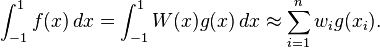
Common weighting functions include  (Gauss-Chebyshev) and
 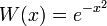 (Gauss-Hermite).
(Gauss-Chebyshev) and (Gauss-Hermite).
It can be shown (see Press, et al., or Stoer and Bulirsch) that the evaluation points are just the roots of a polynomial belonging to a class of orthogonal polynomials.
Contents[hide] |
[edit]Rules for the basic problem
For the integration problem stated above, the associated polynomials are Legendre polynomials, Pn(x). With the nth polynomial normalized to give Pn(1) = 1, the ith Gauss node, xi, is the ith root of Pn; its weight is given by (Abramowitz & Stegun 1972, p. 887)
![w_i = \frac{2}{\left( 1-x_i^2 \right) [P'_n(x_i)]^2} \,\!](http://upload.wikimedia.org/math/c/a/c/caca349155d20da24e3107d74d4d4f03.png)
Some low-order rules for solving the integration problem are listed below.
| Number of points, n | Points, xi | Weights, wi |
|---|---|---|
| 1 | 0 | 2 |
| 2 |  | 1 |
| 3 | 0 | 8⁄9 |
 | 5⁄9 | |
| 4 |  |  |
 |  | |
| 5 | 0 | 128⁄225 |
 |  | |
 |  |
[edit]Change of interval for Gaussian quadrature
An integral over [a, b] must be changed into an integral over [−1, 1] before applying the Gaussian quadrature rule. This change of interval can be done in the following way:

After applying the Gaussian quadrature rule, the following approximation is:

[edit]Other forms
The integration problem can be expressed in a slightly more general way by introducing a positive weight function ω into the integrand, and allowing an interval other than [−1, 1]. That is, the problem is to calculate
for some choices of a, b, and ω. For a = −1, b = 1, and ω(x) = 1, the problem is the same as that considered above. Other choices lead to other integration rules. Some of these are tabulated below. Equation numbers are given for Abramowitz and Stegun(A & S).
| Interval | ω(x) | Orthogonal polynomials | A & S | For more information, see ... |
|---|---|---|---|---|
| [−1, 1] |  | Legendre polynomials | 25.4.29 | Section Rules for the basic problem, above |
| (−1, 1) |  | Jacobi polynomials | 25.4.33 (β = 0) | |
| (−1, 1) |  | Chebyshev polynomials (first kind) | 25.4.38 | Chebyshev–Gauss quadrature |
| [−1, 1] |  | Chebyshev polynomials (second kind) | 25.4.40 | Chebyshev–Gauss quadrature |
| [0, ∞) |  | Laguerre polynomials | 25.4.45 | Gauss–Laguerre quadrature |
| (−∞, ∞) |  | Hermite polynomials | 25.4.46 | Gauss–Hermite quadrature |
[edit]Fundamental theorem
Let pn be a nontrivial polynomial of degree n such that

If we pick the n nodes xi to be the zeros of pn , then there exist n weights wi which make the Gauss-quadrature computed integral exact for all polynomials h(x) of degree 2n − 1 or less. Furthermore, all these nodes xi will lie in the open interval (a, b) (Stoer & Bulirsch 2002, pp. 172–175).
The polynomial pn is said to be an orthogonal polynomial of degree n associated to the weight function ω(x). It is unique up to a constant normalization factor. The idea underlying the proof is that, because of its sufficiently low degree, h(x) can be divided by pn(x) to produce quotient q(x) and remainder r(x), both latter polynomials which will have degree strictly lower than n, so that both will be orthogonal to pn(x), by the defining property of pn(x). Thus
 .
.
Because of the choice of nodes xi , the corresponding relation

holds also. The exactness of the computed integral for h(x) then follows from corresponding exactness for polynomials of degree only n or less (as is r(x)). This (superficially less exacting) requirement can now be satisfied by choosing the weights wi equal to the integrals (using same weight function ω) of the Lagrange basis polynomials  of these particular n nodes xi.
of these particular n nodes xi.[edit]Computation of Gaussian quadrature rules
For computing the nodes xi and weights wi of Gaussian quadrature rules, the fundamental tool is the three-term recurrence relation satisfied by the set of orthogonal polynomials associated to the corresponding weight function. For n points, these nodes and weights can be computed in O(n2) operations by the following algorithm.
If, for instance, pn is the monic orthogonal polynomial of degree n (the orthogonal polynomial of degree n with the highest degree coefficient equal to one), one can show that such orthogonal polynomials are related through the recurrence relation

From this, nodes and weights can be computed from the eigenvalues and eigenvectors of an associated linear algebra problem. This is usually named as the Golub–Welsch algorithm (Gil, Segura & Temme 2007).
The starting idea comes from the observation that, if xi is a root of the orthogonal polynomial pn then, using the previous recurrence formula for 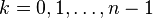 and because pn(xj) = 0, we have
and because pn(xj) = 0, we have
where ![\tilde{P}=[p_0 (x_j),p_1 (x_j),...,p_{n-1}(x_j)]^{T}](http://upload.wikimedia.org/math/e/4/0/e40d7fca88274e88ea1ca5ff6dac2d2e.png)
and J is the so-called Jacobi matrix:

The nodes of gaussian quadrature can therefore be computed as the eigenvalues of a tridiagonal matrix.
For computing the weights and nodes, it is preferable to consider the symmetric tridiagonal matrix  with elements
  and
and 
 and are similar matrices and therefore have the same eigenvalues (the nodes). The weights can be computed from the corresponding eigenvectors: If φ(j) is a normalized eigenvector (i.e., an eigenvector with euclidean norm equal to one) associated to the eigenvalue xj, the corresponding weight can be computed from the first component of this eigenvector, namely:
with elements and and are similar matrices and therefore have the same eigenvalues (the nodes). The weights can be computed from the corresponding eigenvectors: If φ(j) is a normalized eigenvector (i.e., an eigenvector with euclidean norm equal to one) associated to the eigenvalue xj, the corresponding weight can be computed from the first component of this eigenvector, namely:
where μ0 is the integral of the weight function
See, for instance, (Gil, Segura & Temme 2007) for further details.
[edit]Error estimates
The error of a Gaussian quadrature rule can be stated as follows (Stoer & Bulirsch 2002, Thm 3.6.24). For an integrand which has 2n continuous derivatives,

for some ξ in (a, b), where pn is the orthogonal polynomial of degree n and where

In the important special case of ω(x) = 1, we have the error estimate (Kahaner, Moler & Nash 1989, §5.2)
![\frac{(b-a)^{2n+1} (n!)^4}{(2n+1)[(2n)!]^3} f^{(2n)} (\xi) , \qquad a < \xi < b . \,\!](http://upload.wikimedia.org/math/4/9/1/491af0702cc44d4ad5bef4992a40370f.png)
Stoer and Bulirsch remark that this error estimate is inconvenient in practice, since it may be difficult to estimate the order 2n derivative, and furthermore the actual error may be much less than a bound established by the derivative. Another approach is to use two Gaussian quadrature rules of different orders, and to estimate the error as the difference between the two results. For this purpose, Gauss–Kronrod quadrature rules can be useful.
Important consequence of the above equation is that Gaussian quadrature of order n is accurate for all polynomials up to degree 2n–1.
[edit]Gauss–Kronrod rules
Main article: Gauss–Kronrod quadrature formula
If the interval [a, b] is subdivided, the Gauss evaluation points of the new subintervals never coincide with the previous evaluation points (except at zero for odd numbers), and thus the integrand must be evaluated at every point. Gauss–Kronrod rules are extensions of Gauss quadrature rules generated by adding n + 1 points to an n-point rule in such a way that the resulting rule is of order 3n + 1. This allows for computing higher-order estimates while re-using the function values of a lower-order estimate. The difference between a Gauss quadrature rule and its Kronrod extension are often used as an estimate of the approximation error.
[edit]Gauss–Lobatto rules
Also known as Lobatto quadrature (Abramowitz & Stegun 1972, p. 888), named after Dutch mathematician Rehuel Lobatto.
It is similar to Gaussian quadrature with the following differences:
- The integration points include the end points of the integration interval.
- It is accurate for polynomials up to degree 2n–3, where n is the number of integration points.
Lobatto quadrature of function f(x) on interval [–1, +1]:
![\int_{-1}^1 {f(x) \, dx} =
\frac {2} {n(n-1)}[f(1) + f(-1)] +
\sum_{i = 2} ^{n-1} {w_i f(x_i)} + R_n.](http://upload.wikimedia.org/math/c/7/7/c77f8162f24ddb8dddcdd5f2e81da912.png)
Abscissas: xi is the (i − 1)st zero of P'n − 1(x).
Weights:
![w_i = \frac{2}{n(n-1)[P_{n-1}(x_i)]^2} \quad (x_i \ne \pm 1).](http://upload.wikimedia.org/math/d/c/6/dc60d6086449b1dde8c7d5ce3638684f.png)
Remainder: ![R_n = \frac
{- n (n-1)^3 2^{2n-1} [(n-2)!]^4}
{(2n-1) [(2n-2)!]^3}
f^{(2n-2)}(\xi), \quad (-1 < \xi < 1)](http://upload.wikimedia.org/math/9/c/4/9c457ec6355ccc218cfdca0899e342eb.png)
[edit]References
- Abramowitz, Milton; Stegun, Irene A., eds. (1972), "§25.4, Integration", Handbook of Mathematical Functions (with Formulas, Graphs, and Mathematical Tables), Dover, ISBN 978-0-486-61272-0
- Gil, Amparo; Segura, Javier; Temme, Nico M. (2007), "§5.3: Gauss quadrature", Numerical Methods for Special Functions, SIAM, ISBN 978-0-898716-34-4
- Golub, Gene H.; Welsch, John H. (1969), "Calculation of Gauss Quadrature Rules", Mathematics of Computation 23 (106): 221–230, JSTOR 2004418
- Kahaner, David; Moler, Cleve; Nash, Stephen (1989), Numerical Methods and Software, Prentice-Hall, ISBN 978-0-13-627258-8
- Press, William H.; Flannery, Brian P.; Teukolsky, Saul A.; Vetterling, William T. (1988), "§4.5: Gaussian Quadratures and Orthogonal Polynomials", Numerical Recipes in C (2nd ed.), Cambridge University Press, ISBN 978-0-521-43108-8
- Stoer, Josef; Bulirsch, Roland (2002), Introduction to Numerical Analysis (3rd ed.), Springer, ISBN 978-0-387-95452-3.
- Temme, Nico M. (2010), "§3.5(v): Gauss Quadrature", in Olver, Frank W. J.; Lozier, Daniel M.; Boisvert, Ronald F. et al., NIST Handbook of Mathematical Functions, Cambridge University Press, ISBN 978-0521192255
[edit]External links
- ALGLIB contains a collection of algorithms for numerical integration (in C# / C++ / Delphi / Visual Basic / etc.)
- GNU Scientific Library - includes C version of QUADPACK algorithms (see also GNU Scientific Library)
- From Lobatto Quadrature to the Euler constant e
- Gaussian Quadrature Rule of Integration - Notes, PPT, Matlab, Mathematica, Maple, Mathcad at Holistic Numerical Methods Institute
- Gaussian Quadrature table at sitmo.com
- Legendre-Gauss Quadrature at MathWorld
- Gaussian Quadrature by Chris Maes and Anton Antonov, Wolfram Demonstrations Project.
- High-precision abscissas and weights for Gaussian Quadrature for n = 2, ..., 20, 32, 64, 100, 128, 256, 512, 1024 also contains C language source code under LGPL license.
[edit]See also
Legendre polynomials
From Wikipedia, the free encyclopedia
For Legendre's Diophantine equation, see Legendre's equation.
- Note: Associated Legendre polynomials is the most general solution to Legendre's Equation and 'Legendre polynomials' are solutions that are azimuthally symmetric i.e. m=0.
In mathematics, Legendre functions are solutions to Legendre's differential equation:
![{d \over dx} \left[ (1-x^2) {d \over dx} P_n(x) \right] + n(n+1)P_n(x) = 0.](http://upload.wikimedia.org/math/5/2/b/52bff80109b66b45a6fb0ea62522a03f.png)
They are named after Adrien-Marie Legendre. This ordinary differential equation is frequently encountered in physics and other technical fields. In particular, it occurs when solving Laplace's equation (and related partial differential equations) in spherical coordinates.
The Legendre differential equation may be solved using the standard power series method. The equation has regular singular points at x = ±1 so, in general, a series solution about the origin will only converge for |x| < 1. When n is an integer, the solutionPn(x) that is regular at x = 1 is also regular at x = −1, and the series for this solution terminates (i.e. is a polynomial).
These solutions for n = 0, 1, 2, ... (with the normalization Pn(1) = 1) form a polynomial sequence of orthogonal polynomials called the Legendre polynomials. Each Legendre polynomial Pn(x) is an nth-degree polynomial. It may be expressed usingRodrigues' formula:
![P_n(x) = {1 \over 2^n n!} {d^n \over dx^n } \left[ (x^2 -1)^n \right].](http://upload.wikimedia.org/math/7/0/a/70a1790c4fb6b05d9ccea331b0dabe51.png)
That these polynomials satisfy the Legendre differential equation (1) follows by differentiating (n+1) times both sides of the identity

and employing the general Leibniz rule for repeated differentiation.[1] The Pn can also be defined as the coefficients in a Taylor series expansion:[2]
 .
.
In physics, this generating function is the basis for multipole expansions.
Contents[hide] |
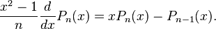
[edit]Recursive Definition
Expanding the Taylor series in equation (1) for the first two terms gives

for the first two Legendre Polynomials. To obtain further terms without resorting to direct expansion of the Taylor series, equation (1) is differentiated with respect to t on both sides and rearranged to obtain

Replacing the quotient of the square root with its definition in (1), and equating the coefficients of powers of t in the resulting expansion gives Bonnet’s recursion formula

This relation, along with the first two polynomials P0 and P1, allows the Legendre Polynomials to be generated recursively.
The first few Legendre polynomials are:
| n |  |
| 0 | |
| 1 |  |
| 2 |  |
| 3 |  |
| 4 |  |
| 5 |  |
| 6 |  |
| 7 |  |
| 8 |  |
| 9 |  |
| 10 |  |
The graphs of these polynomials (up to n = 5) are shown below:

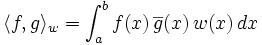
[edit]The orthogonality property
An important property of the Legendre polynomials is that they are orthogonal with respect to the L2 inner product on the interval −1 ≤ x ≤ 1:

(where δmn denotes the Kronecker delta, equal to 1 if m = n and to 0 otherwise). In fact, an alternative derivation of the Legendre polynomials is by carrying out the Gram-Schmidt process on the polynomials {1, x, x2, ...} with respect to this inner product. The reason for this orthogonality property is that the Legendre differential equation can be viewed as a Sturm–Liouville problem, where the Legendre polynomials are eigenfunctions of a Hermitian differential operator:
![{d \over dx} \left[ (1-x^2) {d \over dx} P(x) \right] = -\lambda P(x),](http://upload.wikimedia.org/math/b/9/3/b93b0519eba36d1149a5ad46e123f14d.png)
where the eigenvalue λ corresponds to n(n + 1).
[edit]Applications of Legendre polynomials in physics
The Legendre polynomials were first introduced in 1782 by Adrien-Marie Legendre[3] as the coefficients in the expansion of the Newtonian potential

where r and r' are the lengths of the vectors  and
and  respectively and γ is the angle between those two vectors. The series converges when r > r'. The expression gives the gravitational potential associated to a point mass or the Coulomb potentialassociated to a point charge. The expansion using Legendre polynomials might be useful, for instance, when integrating this expression over a continuous mass or charge distribution.
and respectively and γ is the angle between those two vectors. The series converges when r > r'. The expression gives the gravitational potential associated to a point mass or the Coulomb potentialassociated to a point charge. The expansion using Legendre polynomials might be useful, for instance, when integrating this expression over a continuous mass or charge distribution.
Legendre polynomials occur in the solution of Laplace equation of the potential,  , in a charge-free region of space, using the method of separation of variables, where the boundary conditions have axial symmetry (no dependence on anazimuthal angle). Where
  is the axis of symmetry and θ is the angle between the position of the observer and the axis (the zenith angle), the solution for the potential will be
, in a charge-free region of space, using the method of separation of variables, where the boundary conditions have axial symmetry (no dependence on anazimuthal angle). Where is the axis of symmetry and θ is the angle between the position of the observer and the axis (the zenith angle), the solution for the potential will be![\Phi(r,\theta)=\sum_{\ell=0}^{\infty} \left[ A_\ell r^\ell + B_\ell r^{-(\ell+1)} \right] P_\ell(\cos\theta).](http://upload.wikimedia.org/math/d/3/a/d3a683c19b5e5e533d574488ec388893.png)
 and
and  are to be determined according to the boundary condition of each problem[4].
Legendre polynomials in multipole expansions

Legendre polynomials are also useful in expanding functions of the form (this is the same as before, written a little differently):

which arise naturally in multipole expansions. The left-hand side of the equation is the generating function for the Legendre polynomials.
As an example, the electric potential Φ(r,θ) (in spherical coordinates) due to a point charge located on the z-axis at z = a (Figure 2) varies like

If the radius r of the observation point P is greater than a, the potential may be expanded in the Legendre polynomials

where we have defined η = a/r < 1 and x = cos θ. This expansion is used to develop the normal multipole expansion.
Conversely, if the radius r of the observation point P is smaller than a, the potential may still be expanded in the Legendre polynomials as above, but with a and r exchanged. This expansion is the basis ofinterior multipole expansion.
[edit]Additional properties of Legendre polynomials
Legendre polynomials are symmetric or antisymmetric, that is

Since the differential equation and the orthogonality property are independent of scaling, the Legendre polynomials' definitions are "standardized" (sometimes called "normalization", but note that the actual norm is not unity) by being scaled so that

The derivative at the end point is given by

As discussed above, the Legendre polynomials obey the three term recurrence relation known as Bonnet’s recursion formula

and
Useful for the integration of Legendre polynomials is
![(2n+1) P_n(x) = {d \over dx} \left[ P_{n+1}(x) - P_{n-1}(x) \right].](http://upload.wikimedia.org/math/0/5/1/0514363f3f110b3a86cfc874ef9fcdfe.png)
From the above one can see also that

or equivalently

From Bonnet’s recursion formula one obtains by induction the explicit representation

[edit]Shifted Legendre polynomials
The shifted Legendre polynomials are defined as  . Here the "shifting" function
  (in fact, it is an affine transformation) is chosen such that it bijectively maps the interval [0, 1] to the interval [−1, 1], implying that the polynomials
  are orthogonal on [0, 1]:
. Here the "shifting" function (in fact, it is an affine transformation) is chosen such that it bijectively maps the interval [0, 1] to the interval [−1, 1], implying that the polynomials are orthogonal on [0, 1]:
An explicit expression for the shifted Legendre polynomials is given by

The analogue of Rodrigues' formula for the shifted Legendre polynomials is
![\tilde{P_n}(x) = \frac{1}{n!} {d^n \over dx^n } \left[ (x^2 -x)^n \right].\,](http://upload.wikimedia.org/math/1/1/e/11e6dcc3907748fbb11f4e34bcc636a0.png)
The first few shifted Legendre polynomials are:
| n | |
| 0 | 1 |
| 1 | 2x − 1 |
| 2 | 6x2 − 6x + 1 |
| 3 | 20x3 − 30x2 + 12x − 1 |
[edit]Legendre functions of fractional order
Main article: Legendre function
Legendre functions of fractional order exist and follow from insertion of fractional derivatives as defined by fractional calculus and non-integer factorials (defined by the gamma function) into the Rodrigues' formula. The resulting functions continue to satisfy the Legendre differential equation throughout (−1,1), but are no longer regular at the endpoints. The fractional order Legendre function Pn agrees with the associated Legendre polynomial P0
n.
n.
[edit]See also
- Associated Legendre functions
- Gaussian quadrature
- Gegenbauer polynomials
- Legendre rational functions
- Turán's inequalities
- Legendre wavelet
- Jacobi polynomials
- Spherical Harmonics
[edit]Notes
- ^ Courant & Hilbert 1953, II, §8
- ^ a b George B. Arfken, Hans J. Weber (2005), Mathematical Methods for Physicists, Elsevier Academic Press, p. 743, ISBN 0120598760
- ^ Adrien-Marie Le Gendre, "Recherches sur l'attraction des sphéroïdes homogènes," Mémoires de Mathématiques et de Physique, présentés à l'Académie royale des sciences (Paris) par sçavants étrangers, vol. 10, pages 411-435. [Note: Legendre submitted his findings to the Academy in 1782, but they were published in 1785.] Available on-line (in French) at: http://edocs.ub.uni-frankfurt.de/volltexte/2007/3757/pdf/A009566090.pdf .
- ^ Jackson, J.D. Classical Electrodynamics, 3rd edition, Wiley & Sons, 1999. page 103
[edit]References
- Abramowitz, Milton; Stegun, Irene A., eds. (1965), "Chapter 8", Handbook of Mathematical Functions with Formulas, Graphs, and Mathematical Tables, New York: Dover, pp. 332, MR0167642, ISBN 978-0486612720 See also chapter 22.
- Bayin, S.S. (2006), Mathematical Methods in Science and Engineering, Wiley, Chapter 2.
- Belousov, S. L. (1962), Tables of normalized associated Legendre polynomials, Mathematical tables, 18, Pergamon Press.
- Courant, Richard; Hilbert, David (1953), Methods of Mathematical Physics, Volume 1, New York: Interscience Publischer, Inc.
- Dunster, T. M. (2010), "Legendre and Related Functions", in Olver, Frank W. J.; Lozier, Daniel M.; Boisvert, Ronald F. et al., NIST Handbook of Mathematical Functions, Cambridge University Press, ISBN 978-0521192255
- Koornwinder, Tom H.; Wong, Roderick S. C.; Koekoek, Roelof; Swarttouw, René F. (2010), "Orthogonal Polynomials", in Olver, Frank W. J.; Lozier, Daniel M.; Boisvert, Ronald F. et al., NIST Handbook of Mathematical Functions, Cambridge University Press, ISBN 978-0521192255
- Refaat El Attar (2009), Legendre Polynomials and Functions, CreateSpace, ISBN 978-1441490124
[edit]External links
- A quick informal derivation of the Legendre polynomial in the context of the quantum mechanics of hydrogen
- Wolfram MathWorld entry on Legendre polynomials
- Module for Legendre Polynomials by John H. Mathews
- Dr James B. Calvert's article on Legendre polynomials from his personal collection of mathematics
Generalized Fourier series
From Wikipedia, the free encyclopedia
| This article does not cite any references or sources. Please help improve this article by adding citations to reliable sources. Unsourced material may be challenged and removed. (August 2009) |
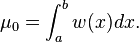
In mathematical analysis, many generalizations of Fourier series have proved to be useful. They are all special cases of decompositions over an orthonormal basis of an inner product space. Here we consider that of square-integrable functions defined on an interval of the real line, which is important, among others, for interpolation theory.
Contents[hide] |
[edit]Definition
Consider a set of square-integrable functions with values in F=C or R,
![\Phi = \{\varphi_n:[a,b]\rightarrow F\}_{n=0}^\infty,](http://upload.wikimedia.org/math/6/d/5/6d50fb34b3b051bfa589dc70e8039a36.png)
which are pairwise orthogonal for the inner product
where w(x) is a weight function, and  represents complex conjugation, i.e.
  for F=R.
represents complex conjugation, i.e. for F=R.
The generalized Fourier series of a square-integrable function f: [a, b] → F, with respect to Φ, is then

where the coefficients are given by
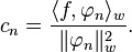
If Φ is a complete set, i.e., an orthonormal basis of the space of all square-integrable functions on [a, b], as opposed to a smaller orthonormal set, the relation  becomes equality in the L² sense, more precisely modulo |·|w (not necessarily pointwise, noralmost everywhere).
becomes equality in the L² sense, more precisely modulo |·|w (not necessarily pointwise, noralmost everywhere).[edit]Example (Fourier–Legendre series)
The Legendre polynomials are solutions to the Sturm–Liouville problem

and because of the theory, these polynomials are eigenfunctions of the problem and are solutions orthogonal with respect to the inner product above with unit weight. So we can form a generalized Fourier series (known as a Fourier–Legendre series) involving the Legendre polynomials, and

As an example, let us calculate the Fourier–Legendre series for ƒ(x) = cos x over [−1, 1]. Now,

and a series involving these terms


which differs from cos x by approximately 0.003, about 0. It may be advantageous to use such Fourier–Legendre series since the eigenfunctions are all polynomials and hence the integrals and thus the coefficients are easier to calculate.
[edit]Coefficient theorems
Some theorems on the coefficients cn include:
[edit]Bessel's inequality
[edit]Parseval's theorem
If Φ is a complete set,

[edit]See also

Thank you very much and hope this article will be useful to you!!!
ANOTHER ORTHOGONAL SIMPLISTIC APPROACH TO COMPRESSING DATA SENDING JUST THE EIGENVALUES OF THE EIGENVECTORS OF AN EUCLIDEAN SPACE NxN MATRIX.
Just by thinking a little bit i found a linnear example that resulst in a quickest calculation way.the idea is very simplistic and based in the diagonal expression of a N equations of N terms in an appropiate Base space.
thus we have the packet of data composed bya matrix
A=(a00 a10 a20 a30...an0)
(a01 a11 a21 a31..an1)
(..................................)
(a0n an1 an2 an3..ann) the biggest the matrix higher compression its reached the rate of compression is by (N-1)*N kb per N kb
the matrix A is in base (e0,e1,..,en)in another euclidean base B can be expressed as BAB^-1=(lambdai) diagonal matrix
=BAB^t/B=(lambda1,lambda2,lambda3,..,lambdan)*I where I is the identity matrix and we also have the fact that |A-lambda*I|=0 and
B^-1*(lambda1,lambda2,lambda3,..,lambdan)*I*B=B^t*B/B*(lambda)=B^t*(lambda)=A
|(enn 0 ..0..0.....0|lambda1 0 0 0)|
|(0 e(n-1)(n-1) 0| 0 lambda2 0 0)|=0
|(... ... ... ... | 0 0 ............... 0)|
|(0.. 0. ... 0 ... e0 | 0 0 0 lambdan)|
wich is the compressing/decompressing varmonde determinant
so for any linear combination of rows and columns with lambdai=A
we obtain a linear combination of the base (e1,e2,..,en) base B can be rewritten from base lambda thus e1+e2=d1,e3+e6-e2=d2...e5+e2-e1=dn for example.
so for data sent into a matrix m>n x n in wich the new subpacket (row or column) is a linnear combination of others can be simplified and begun compresed indicating the linear combination of the basesubi and the eigenvalue lambda
happy compressing!!
thus for any linnear combination of |A-lambda*I|=0
|(enn 0 ..0..0.....0|lambda1 0 0 0)|
|(0 e(n-1)(n-1) 0| 0 lambda2 0 0)|=0
|(... ... ... ... | 0 0 ............... 0)|
|(0.. 0. ... 0 ... e0 | 0 0 0 lambdan)|
|( 1 1 0 1 |= (enn +e(n-1)+e0)*1 -> this byte can be precalc
|(a00 0 ..0..0.....0|lambda1 0 0 0)|
|(0 a(11)0 0| 0 lambda2 0 0)|=|A|
|(... ... ... ... | 0 0 ............... 0)|
|(0.. 0. ... 0 ... ann| 0 0 0 lambdan)|
|( 1 1 0 1 |= (enn +e(n-1)+e0)*1 -> this byte can be precalc
|(enn 0 ..0..0.....0|b00a00bnn/b00.0 0 0)|
|(0 e(n-1)(n-1) 0| 0 b11a00b(n-1)(n-1)/b11 0 0)|=I
|(... ... ... ... | 0 0 ..,,,,,,,,,,,,,,,. ............ 0)|
|(0.. 0. ... 0 ... e0 | 0 0 0 bnnannb00/bnn)|
|( 1 1 0 1 |= (enn +e(n-1)+e0)*1 -> this byte can be precalc
another interesting option is to calc in base the previous compresed rows in based a recurrence i.e enn=e(n-1)-e(n-2)/e1n etc just use your imagination there are infinite possibilities!!!
Yours Sincerely. David
-------------------------------------------------------------------------------------------------------------
MIT article securoty and RSA ( the base of https:// protocol)


-------------------------------------------------------------------------------------------------------------
MIT article securoty and RSA ( the base of https:// protocol)
Rivest unlocks cryptography's past, looks toward future
Public-key system has worked and made Internet commerce feasible, but new systems are ready in case flaws are found.
The most widely used cryptographic system today may eventually be vulnerable, said computer science professor Ronald Rivest — one of the system's primary creators — but even if it fails, new systems are already waiting to be deployed.
Rivest, the Andrew and Erna Viterbi Professor of Computer Science, reviewed the history of code-making and code-breaking through the ages — the field known as cryptography — and made some predictions about the field’s future during MIT's prestigious Killian Faculty Achievement Award Lecture, held on Tuesday, Feb. 8.
The cryptographic system currently used for the vast majority of all financial transactions and secure communications over the Internet was developed in 1977 by Rivest and two of his colleagues — professors Adi Shamir and Len Adleman of MIT’s mathematics department — and is known by their initials: RSA. The system depends on the fact that it is extremely difficult and time consuming to determine the prime factors of a large number (the prime numbers that can be multiplied together to produce the given number).
But Rivest said that it has not been shown mathematically that such factorization into primes is necessarily difficult. “Factoring could turn out to be easy,” Rivest said. So it remains possible, he told the audience, that “maybe someone here will find the method” that renders the RSA encryption system vulnerable, in which case companies would be forced to switch quickly to some other encryption system. Fortunately, he said, a variety of alternative schemes have been developed in the decades since RSA was published, and a new system could probably be adopted quickly.
RSA is an example of a “public key” code system, in which one key is used to encrypt a message, and another key is used to decrypt an encrypted text. One of those keys is publicly known, but it nevertheless is extremely difficult to discover the other key. The concept of public-key codes was developed and published by researchers at Stanford in 1976, who declared that “we are at the brink of a revolution in cryptography.” However, Rivest said, “they didn’t know how to implement them at all.” Rivest and his colleagues were the first to translate the concept into a practical, workable system, and they founded a company in 1982, RSA Data Security, to commercialize it. The company was ultimately sold to EMC Corp.
At the time, there was little interest or active research on factoring, Rivest said. But when they came up with their encryption system, Martin Gardner wrote a column about it in Scientific American and offered a challenge: a $100 reward for the first person to find the prime factors of a 129-digit number he published. Rivest at the time estimated that the puzzle would take 40 quadrillion years to solve. That proved to be a bit of an overestimate, he acknowledged: It was solved 17 years later, in a group effort involving 8 months of work by 600 volunteers — and Rivest cheerfully paid up the $100.
While early codes go back at least as far as the ancient civilizations of Egypt and Greece — one early version used a strip of paper that had to be wound around a stick of a specific diameter in order for the letters to line up so a message could be read — it is advances in technology that have provided the impetus for more advanced code systems, Rivest said. For example, it was the spread of radio in the 20th century that made new codes imperative, and mechanical coding and decoding devices became a key factor on both sides during World War II. Then, with the creation of the World Wide Web in the 1990s, the need for stronger and easier-to-implement codes became significant.
For example, one spinoff of technology related to the RSA system is the digital certificate company VeriSign, which uses digital signatures, a concept also developed by some of the same researchers, to authenticate the identity of websites. The company now provides 1.3 billion certificate authentications every day, he said.
In theory, a newer technology could render RSA useless, Rivest said. A large quantum computer — if one is ever built — could theoretically factor numbers quickly enough to defeat the code. On the other hand, he said, there’s not likely to be any motivation for building such a complex device, since it might have no other real purpose than defeating RSA — and once it was in existence, everyone would stop using RSA, so “there would be no use for it anymore.”
In the meantime, the whole field of cryptography has really taken off, with real or potential applications in such areas as the creation of a secure micropayment system, although such a system developed by Rivest in 2001, called Peppercoin, never got off the ground. Another possible application is secure voting, such as a system that allows a voter to confirm online that his or her vote was correctly tallied, without allowing anyone else to determine which candidate was voted for.
Ironically, Rivest said, the development of such a secure, verifiable cryptographic system for voting verification “actually increases transparency and verifiability,” by allowing individual voters to check their own votes, while also providing a paper trail for possible recounts. Developing a secure voting system that meets all the different requirements for such a system — including allowing voters to verify their votes, but without making it possible for them to sell their votes, and while achieving a high degree of usability — remains a tough technical challenge. “We’ll get there,” he said, “but there’s work to be done.”
As an area of research, Rivest said, cryptography remains an active and fascinating area, one that brings together disciplines as varied as mathematics, statistics, theoretical computer science, electronic engineering and even psychology. “It’s like the Middle East of research,” he said, “because everything goes through it.”
multimedia
Ronald Rivest, the Andrew and Erna Viterbi Professor of Computer Science.
related
tags
awards and honors
computer science and artificial intelligence laboratory
computer science and technology
cryptography
faculty
special events and guest speakers
RSA
En criptografía, RSA (Rivest, Shamir y Adleman) es un sistema criptográfico de clave pública desarrollado en 1977. En la actualidad, RSA es el primer y más utilizado algoritmo de este tipo y es válido tanto para cifrar como para firmar digitalmente.
La seguridad de este algoritmo radica en el problema de la factorización de números enteros. Los mensajes enviados se representan mediante números, y el funcionamiento se basa en el producto, conocido, de dos números primos grandes elegidos al azar y mantenidos en secreto. Actualmente estos primos son del orden de 10200, y se prevé que su tamaño aumente con el aumento de la capacidad de cálculo de los ordenadores.
Como en todo sistema de clave pública, cada usuario posee dos claves de cifrado: una pública y otra privada. Cuando se quiere enviar un mensaje, el emisor busca la clave pública del receptor, cifra su mensaje con esa clave, y una vez que el mensaje cifrado llega al receptor, este se ocupa de descifrarlo usando su clave privada.
Se cree que RSA será seguro mientras no se conozcan formas rápidas de descomponer un número grande en producto de primos. La computación cuántica podría proveer de una solución a este problema de factorización.
Contenido[ocultar] |
[editar]Historia
El algoritmo fue descrito en 1977 por Ron Rivest, Adi Shamir y Len Adleman, del Instituto Tecnológico de Massachusetts (MIT); las letras RSA son las iniciales de sus apellidos. Clifford Cocks, un matemático británico que trabajaba para la agencia de inteligencia británica GCHQ, había descrito un sistema equivalente en un documento interno en 1973. Debido al elevado coste de las computadoras necesarias para implementarlo en la época su idea no trascendió. Su descubrimiento, sin embargo, no fue revelado hasta 1997 ya que era confidencial, por lo que Rivest, Shamir y Adleman desarrollaron RSA de forma independiente.
El algoritmo fue patentado por el MIT en 1983 en Estados Unidos con el número 4.405.829. Esta patente expiró el 21 de septiembre de 2000. Como el algoritmo fue publicado antes de patentar la aplicación, esto impidió que se pudiera patentar en otros lugares del mundo. Dado que Cocks trabajó en un organismo gubernamental, una patente en Estados Unidos tampoco hubiera sido posible.
[editar]Algoritmo RSA
El algoritmo consta de tres pasos: generación de claves, cifrado y descifrado.
[editar]Idea del algoritmo
Alicia envía a Bob una caja con una cerradura abierta, de la que solo Alicia tiene la llave. Bob recibe la caja, escribe el mensaje, lo pone en la caja y la cierra con su cerradura (ahora Bob no puede leer el mensaje). Bob envía la caja a Alicia y ella la abre con su llave. En este ejemplo, la caja con la cerradura es la «clave pública» de Alicia, y la llave de la cerradura es su «clave privada».
Técnicamente, Bob envía a Alicia un «mensaje llano» M en forma de un número m menor que otro número n, mediante un protocolo reversible conocido como padding scheme («patrón de relleno»). A continuación genera el «mensaje cifrado» c mediante la siguiente operación:
 ,
,
donde e es la clave pública de Alicia.
Ahora Alicia descifra el mensaje en clave c mediante la operación inversa dada por
 ,
,
donde d es la clave privada que solo Alicia conoce.
[editar]Generación de claves
- Cada usuario elige dos números primos distintos p y q.
- Por motivos de seguridad, estos números deben escogerse de forma aleatoria y deben tener una longitud en bits parecida. Se pueden hallar primos fácilmente mediante test de primalidad.
- Se calcula n = pq.
- n se usa como el módulo para ambas claves, pública y privada.
- Se calcula
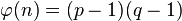 , donde
  es la función φ de Euler.
 - Se escoge un entero positivo e menor que
 , que sea coprimo con .
- e se da a conocer como el exponente de la clave pública.
- Si se escoge un e con una suma encadenada corta, el cifrado será más efectivo. Un exponente e muy pequeño (p. ej. e = 3) podría suponer un riesgo para la seguridad.1
- Se determina un d (mediante aritmética modular) que satisfaga la congruencia
 .
.- Expresado de otra manera, de − 1 es dividido exactamente por .
- Esto suele calcularse mediante el algoritmo de Euclides extendido.
- d se guarda como el exponente de la clave privada.
- Expresado de otra manera, de − 1 es dividido exactamente por
La clave pública es (n,e), esto es, el módulo y el exponente de cifrado. La clave privada es (n,d), esto es, el módulo y el exponente de descifrado, que debe mantenerse en secreto.
Nota:
- PKCS#1 v2.0 y PKCS#1 v2.1 se especifican mediante la función de Carmichael λ(n) = mcm(p − 1,q − 1) en vez de la función φ de Euler, donde mcm es el mínimo común múltiplo.
- Para una mayor eficiencia los siguientes valores se calculan de antemano y se almacenan como parte de la clave privada:
- p y q: los primos para la generación de las claves,
 y
y  ,
,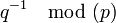 .
.
[editar]Cifrado
Alicia comunica su clave pública (n,e) a Bob y guarda la clave privada en secreto. Ahora Bob desea enviar un mensaje M a Alicia.
Primero, Bob convierte M en un número entero m menor que n mediante un protocolo reversible acordado de antemano. Luego calcula el texto cifrado c mediante la operación
- .
Esto puede hacerse rápido mediante el método de exponenciación binaria. Ahora Bob transmite c a Alicia.
[editar]Descifrado
Alicia puede recuperar m a partir de c usando su exponente d de la clave privada mediante el siguiente cálculo:
- .
Ahora que tiene m en su poder, puede recuperar el mensaje original M invirtiendo el padding scheme.
El procedimiento anterior funciona porque
 .
.
Esto es así porque, como hemos elegido d y e de forma que 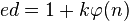 , se cumple
, se cumple .
.
La última congruencia se sigue directamente del teorema de Euler cuando m es coprimo con n. Puede demostrarse que las ecuaciones se cumplen para todo m usando congruencias y el teorema chino del resto.
Esto muestra que se obtiene el mensaje original:
- .
[editar]Ejemplo
Aquí tenemos un ejemplo de cifrado/descifrado con RSA. Los parámetros usados aquí son pequeños y orientativos con respecto a los que maneja el algoritmo, pero podemos usar también OpenSSL para generar y examinar una par de claves reales.
| p=61 | 1º nº primo Privado |
| q=53 | 2º nº primo Privado |
| n=pq=3233 | producto p*q |
| e=17 | exponente Público |
| d=2753 | exponente Privado |
La clave pública (e, n). La clave privada es d. La función de cifrado es:
-
- encrypt(m) = me(mod n) = m17(mod 3233)
Donde m es el texto sin cifrar. La función de descifrado es:
-
- decrypt(c) = cd(mod n) = c2753(mod 3233)
Donde c es el texto cifrado. Para cifrar el valor del texto sin cifrar 123, nosotros calculamos:
-
- encrypt(123) = 12317(mod 3233) = 855
Para descifrar el valor del texto cifrado, nosotros calculamos:
-
- decrypt(855) = 8552753(mod 3233) = 123
Ambos de estos cálculos pueden ser eficientemente usados por el algoritmo de multiplicación cuadrática para exponenciación modular.
[editar]Padding schemes (Esquema de relleno)
RSA debe ser combinado con alguna versión del padding scheme, ya que si no el valor de M puede llevar a textos cifrados inseguros. RSA usado sin padding scheme podría sufrir muchos problemas.
-
- El valor m=0 o m=1 siempre produce textos cifrados iguales para 0 o 1 respectivamente, debido a propiedades de los exponentes.
- Cuando ciframos con exponentes pequeños (e=3) y valores pequeños de m, el resultado de m podría ser estrictamente menor que el módulo de n. En este caso, el texto cifrado podría ser fácilmente descifrado, tomando la raíz e-ésima del texto cifrado sin tener en cuenta el módulo.
-
- Dado que el cifrado RSA es un algoritmo determinista (no tiene componentes aleatorios) un atacante puede lanzar con éxito un ataque de texto elegido contra el criptosistema, construyendo un diccionario de textos probables con la llave pública, y almacenando el resultado cifrado. Observando los textos cifrados en un canal de comunicación, el atacante puede usar este diccionario para descifrar el contenido del mensaje.
En la práctica, el primero de los dos problemas podría presentarse cuando enviamos pequeños mensajes ASCII donde m es la concatenación de uno o más carácter/es ASCII codificado/s. Un mensaje consiste en un solo carácter ASCII NUL (cuyo valor es 0) se codificaría como m=0, produciendo un texto cifrado de 0 sin importar qué valores de e y N son usados. Probablemente, un solo ASCII SOH (cuyo valor es 1) produciría siempre un texto cifrado de 1. Para sistemas convencionales al usar valores pequeños de e, como 3, un solo carácter ASCII mensaje codificado usando este esquema sería inseguro, ya que el máximo valor de m sería 255, y 255³ es menor que cualquier módulo razonable. De esta manera los textos sin cifrar podrían ser recuperados simplemente tomando la raíz cúbica del texto cifrado. Para evitar estos problemas, la implementación práctica del RSA se ayuda de algunas estructuras, uso del randomized padding dentro del valor de m antes del cifrado. Esta técnica asegura que m no caerá en el rango de textos sin cifrar inseguros, y que dado un mensaje, una vez que este rellenado, cifrará uno de los números grandes de los posibles textos cifrados. La última característica es la incrementación del diccionario haciendo este intratable a la hora de realizar un ataque.
Estándares como PKCS han sido cuidadosamente diseñados para la seguridad de los de mensajes importantes con el cifrado RSA. Porque el pad scheme rellena el texto sin cifrar m con algunos números adicionales (bits); el tamaño del mensaje un-padded M debe ser algo más pequeño. RSA-padding scheme debe ser cuidadosamente diseñado así como para prevenir ataques sofisticados los cuales podrían ser facilitados por la predictibilidad de la estructura del mensaje. Versiones más recientes del PKCS Standard usando construcciones ad-hoc, las cuales fueron encontradas vulnerabilidades más tarde en la practica adaptativa de elección de ataques de textos cifrados. Las construcciones modernas usan técnicas seguras como Optimal Asymetric Encryption Padding (OAEP) para proteger los mensajes mientras previenen estos ataques. El PKCS estándar también incorpora procesado de esquemas diseñados para proveer adicionalmente la seguridad de autentificaciones RSA. Por ejemplo: the Probabilistic Signature Scheme for RSA (RSA-PSS).
[editar]Autenticación de mensajes
RSA puede también ser usado para autenticar un mensaje. Supongamos que Alicia desea enviar un mensaje autentificado a Bob. Ella produce un valor hash del mensaje, lo eleva a la potencia de d≡ mod n (como ella hace cuando descifra mensajes), y lo adjunta al mensaje como una “firma”. Cuando Bob recibe el mensaje autentificado, utiliza el mismo algoritmo hash en conjunción con la clave pública de Alice. Eleva la firma recibida a la potencia de e≡ mod n (como hace cuando cifra mensajes), y compara el resultado hash obtenido con el valor hash del mensaje. Si ambos coinciden, él sabe que el autor del mensaje estaba en posesión de la clave secreta de Alicia, y que el mensaje no ha sido tratado de forzar (no ha sufrido ataques).
Se debe observar que la seguridad de los padding-schemes como RSA-PSS son esenciales tanto para la seguridad de la firma como para el cifrado de mensajes, y que nunca se debería usar la misma clave para propósitos de cifrado y de autentificación.
[editar]Seguridad
La seguridad del criptosistema RSA está basado en dos problemas matemáticos: el problema de factorizar números grandes y el problema RSA. El descifrado completo de un texto cifrado con RSA es computacionalmente intratable, no se ha encontrado un algoritmo eficiente todavía para ambos problemas. Proveyendo la seguridad contra el descifrado parcial podría requerir la adición de una seguridad padding scheme.
El problema del RSA se define como la tarea de tomar raíces eth módulo a componer n: recuperando un valor m tal que me=c ≡mod n, donde (e, n) es una clave pública RSA y c es el texto cifrado con RSA. Actualmente la aproximación para solventar el problema del RSA es el factor del módulo n. Con la capacidad para recuperar factores primos, un atacante puede computar el exponente secreto d desde una clave pública (e, n), entonces descifra c usando el procedimiento estándar. Para conseguir esto, un atacante factoriza n en p y q, y computa (p-1)(q-1) con lo que le permite determinar d y e. No se ha encontrado ningún método en tiempo polinómico para la factorización de enteros largos. Ver factorización de enteros para la discusión de este problema.
La factorización de números grandes por lo general proponen métodos teniendo 663 bits de longitud usando métodos distribuidos avanzados. Las claves RSA son normalmente entre 1024-2048 bits de longitud. Algunos expertos creen que las claves de 1024 bits podrían comenzar a ser débiles en poco tiempo; con claves de 4096 bits podrían ser rotas en un futuro. Por lo tanto, si n es suficientemente grande el algoritmo RSA es seguro. Si n tiene 256 bits o menos, puede ser factorizado en pocas horas con un computador personal, usando software libre. Si n tiene 512 bits o menos, puede ser factorizado por varios cientos de computadoras como en 1999. Un dispositivo hardware teórico llamado TWIRL descrito por Shamir y Tromer en el 2003 cuestionó a la seguridad de claves de 1024 bits. Es actualmente recomendado que n sea como mínimo de 2048 bits de longitud.
En 1993, Peter Shor publicó su algoritmo, mostrando que una computadora cuántica podría en principio mejorar la factorización en tiempo polinomial, mostrando RSA como un algoritmo obsoleto. Sin embargo, las computadoras cuánticas no se esperan que acaben su desarrollo hasta dentro de muchos años.
[editar]Consideraciones prácticas
[editar]Generación de claves
Buscando números primos grandes p y q por el test de aleatoriedad y realizando tests probabilísticos de primalidad los cuales eliminan virtualmente todos los no-primos (eficientemente).
Los números p y q no deberían ser suficientemente cercanos para que la factorización de Fermat para n sea exitosa. Además, si cualquier p-1 o q-1 tiene sólo factores primos pequeños, n puede ser factorizado rápidamente, con lo que estos valores de p o q deben ser descartados.
Uno no debería emplear un método de búsqueda de primos con el cual dar alguna información cualquiera sobre los primos al atacante. En particular, un buen generador aleatorio de números primos para el comienzo del valor empleado. Observar que el requerimiento esta en ambos ‘aleatorios’ e ‘impredecibles’. Esto no son los mismos criterios; un número podría haber sido elegido por un proceso aleatorio, pero si éste es predecible de cualquier forma (o parcialmente predecible), el método usado resultara una seguridad baja. Por ejemplo: la tabla de números aleatorios de Rand Corp en 1950 podría muy bien ser verdaderamente aleatoria, pero ha sido publicada y a ésta puede acceder el atacante. Si el atacante puede conjeturar la mitad de los dígitos de p o q, él podría rápidamente computar la otra mitad. (Ver Coppersmith en 1997).
Es importante que la clave secreta d sea muy grande. Wiener mostró en 1990 que si p esta entre q y 2q (es típico) y d<n1/4/3, entonces d puede ser computado eficientemente de n y e. Aunque valores de e son bajos como 3 han sido usados en el pasado, los exponentes pequeños en RSA esta actualmente en desuso, por razones incluyendo el unpadded del texto sin cifrar, vulnerabilidad listada sobre 65537 es normalmente usado para el valor de e, considerado demasiado grande para evitar ataques de exponenciación pequeños, de hecho tiene un peso de hamming suficiente para facilitar una exponenciación eficiente
[editar]Velocidad
RSA es mucho más lento que DES y que otros criptosistemas simétricos. En la practica, Bob normalmente cifra mensajes con algoritmos simétricos, cifra la clave simétrica con RSA, y transmite a ambos la clave simétrica RSA-cifrada (es decir la transmite cifrada con RSA) y el mensaje simétricamente-cifrado a Alicia.
Esto plantea además problemas adicionales de seguridad, por ejemplo, es de gran importancia usar un generador aleatorio fuerte para claves simétricas, porque de otra forma Eve (un atacante que quiera averiguar el contenido del mensaje) podría puentearla clave asimétrica de RSA mediante la adivinación de la clave simétrica.
[editar]Distribución de claves
Como todos los cifrados, es importante como se distribuyan las claves públicas del RSA. La distribución de la clave debe ser segura contra un atacante que se disponga a espiar el canal para hacer un ataque de replay. Supongamos Eve (atacante) tiene alguna forma de dar a Bob arbitrariamente claves y hacerle creer que provienen de Alicia. Supongamos que Eve puede interceptar transmisiones entre Alicia y Bob. Eve envía a Bob su propia clave pública, como Bob cree que es de Alicia. Eve puede entonces interceptar cualquier texto cifrado enviado por Bob, descifrarlo con su propia clave secreta, guardar una copia del mensaje, cifrar el mensaje con la clave pública de Alicia, y enviar el nuevo texto cifrado a Alicia. En principio, ni Alicia ni Bob han detectado la presencia de Eve. Contra la defensa de ataques algunos están basados en certificados digitales u otros componentes de infraestructuras de la clave pública.
[editar]Véase también
- Clifford Cocks
- Criptografía asimétrica
- Competición de factorización RSA
- Criptografía cuántica
- Criptología
- Firma digital ciega
- Problema RSA
- Teoría de la complejidad computacional
[editar]Referencias
[editar]Notas al pie
- ↑ Boneh, Dan (1999). «Twenty Years of attacks on the RSA Cryptosystem» (en inglés). Notices of the American Mathematical Society (AMS) 46 (2): pp. 203–213.
[editar]Bibliografía
- R. Rivest, A. Shamir, L. Adleman. A Method for Obtaining Digital Signatures and Public-Key Cryptosystems. Communications of the ACM, Vol. 21 (2), pp.120–126. 1978. Previously released as an MIT "Technical Memo" in April 1977. Initial publication of the RSA scheme.
- Thomas H. Cormen, Charles E. Leiserson, Ronald L. Rivest, and Clifford Stein. Introduction to Algorithms, Second Edition. MIT Press and McGraw-Hill, 2001. ISBN 0-262-03293-7. Section 31.7: The RSA public-key cryptosystem, pp.881–887.
- Wing H. Wong. Timing Attacks on RSA: Revealing Your Secrets through the Fourth Dimension
- An Attack on RSA Digital Signature
[editar]Enlaces externos
- Algoritmo RSA
- Ataques RSA I
- PKCS #1: RSA Cryptography Standard (Sitio oficial de RSA Laboratories )
- A Method for Obtaining Digital Signatures and Public-Key Cryptosystems, El documento de la revista Communications of the ACM, Vol. 21 (2), 1978, páginas 120--126 escrita por R. Rivest, A. Shamir y L. Adleman, Posterior al "Technical Memo" de abril de 1977.
- Una introducción a RSA, M. Griep, Oct. 2002
- Calculadora on-line de encriptación RSA que muestra paso a paso todos los cálculos
-------------------------------------------------------------------------------------------------------------
its just from scratch my idea of how computer networks should join its work to have a perception of a sense.
like human brain. parasympathical system is inteligent so if we refuse a sense due it causes a negative emotion or we accept it (cognitive conductal) it resembles something possitive or just it is indiferent the diferent weights
of the function Biases A,B,C,D,E,F,G,H are adjusted for each magnitude/kind of stimulus imagine a simple sensor network like tonge divided into parts for detecting diferent tastes that we interpret in the diagram way.
Diagram of how is human perception. automatically just a glance spinal reflection system observance network+memory cognitive conditioned observance (includes state of aim) network+logic neuron mirror observance network,trying to explain the self path D;F corresponds to logic neuron mirror network of neurons if we draw a 3d perspective drawing bad we realise from observance if its copied form a picture , then realise that is bad if is not the first time we have made a 3d perspective drawing memory but also form logic lines dont converge in that way of umbral obsevance w1*f(x)>w2*g(x)>w3*z(x)
due we cant see at the same time as we paint our work always relay a bit in short memory at least and then by imitation to how our people work and how we like it we can give an human defect with the proposit of obtaining a nonhyperrealistic result but confortable to the enviroment.
the best zone in spain were spanish where is talked spanish is at Valladolid, but sevillians talk in a more southern accent common south people wayits dependes in the context the functions and the umbrals of the networks as you can see but so predominant values in orders of magnitude can express an unadapted network by any non properly functional deficiency reason.after all the thing should be a correlation between network potentials fighting for an emotion / response i submit the diagram wich i dont know exactly wich is each bias participating

Including emotional intelligence thus cognition+parasympatical neuron system can explain so many diseases motor and fisiology of pshycological ones in a retrofeedback mechanism depicted in the diagrams, note the autoconciousness are just a network mirror neurons connected to parasympathic system
click on left menu roll-left
Aqui os dejo todo tipo de recursos sobre inteligencia artificial los links parecen muchos antiguos y puede que algunos esten desactualizados pero muchos son de lo mas interesante...
y documentacion einfo a lo largo dwe todo el mundo sobre inteligencia artificial
Please add your favourite topic or feedback and i will response!!
ResponderEliminar